def E_kinetic(v: np.ndarray, params: dict) -> np.ndarray:
    """Kinetic energy (translation only): 0.5 * m * v^2."""
    m = params["m"]
    return 0.5 * m * (v ** 2)


def E_potential(x: np.ndarray, params: dict) -> np.ndarray:
    """
    Potential energy stored in the spring.
    Model uses an effective extension u = x / T (T: transmission).
    Ep = 0.5 * k * u^2
    """
    k = params["k"]
    T = params["T"]
    u = x / T
    return 0.5 * k * (u ** 2)


def derivatives(t: float, state: np.ndarray, params: dict) -> np.ndarray:
    """
    ODEs for the system.
    state: [x, v]
    x = generalized coordinate (m)
    v = dx/dt (m/s)
    Returns [dx/dt, dv/dt].
    """
    x, v = state
    m = params["m"]
    k = params["k"]
    T = params["T"]

    # spring extension (effective)
    u = x / T
    F_spring = -k * u
    # transmitted force divided by transmission lever T gives acceleration input to mass
    a = (F_spring / T) / m
    return np.array([v, a])


def simulate_system(
    params: dict,
    state0: Tuple[float, float],
    t_span: Tuple[float, float],
    n_frames: int = 300,
) -> Tuple[np.ndarray, np.ndarray]:
    """Simulate system using solve_ivp and return (t, y) where y.shape == (2, len(t))."""
    t_eval = np.linspace(t_span[0], t_span[1], n_frames)
    sol = solve_ivp(
        fun=lambda t, y: derivatives(t, y, params),
        t_span=t_span,
        y0=np.array(state0),
        t_eval=t_eval,
    )
    return sol.t, sol.y


def compute_energies(states: np.ndarray, params: dict) -> Tuple[np.ndarray, np.ndarray]:
    """
    Vectorized energy calculations.
    states: shape (2, N) with rows [x, v]
    Returns (Ekin_array, Epot_array)
    """
    x = states[0, :]
    v = states[1, :]
    return E_kinetic(v, params), E_potential(x, params)


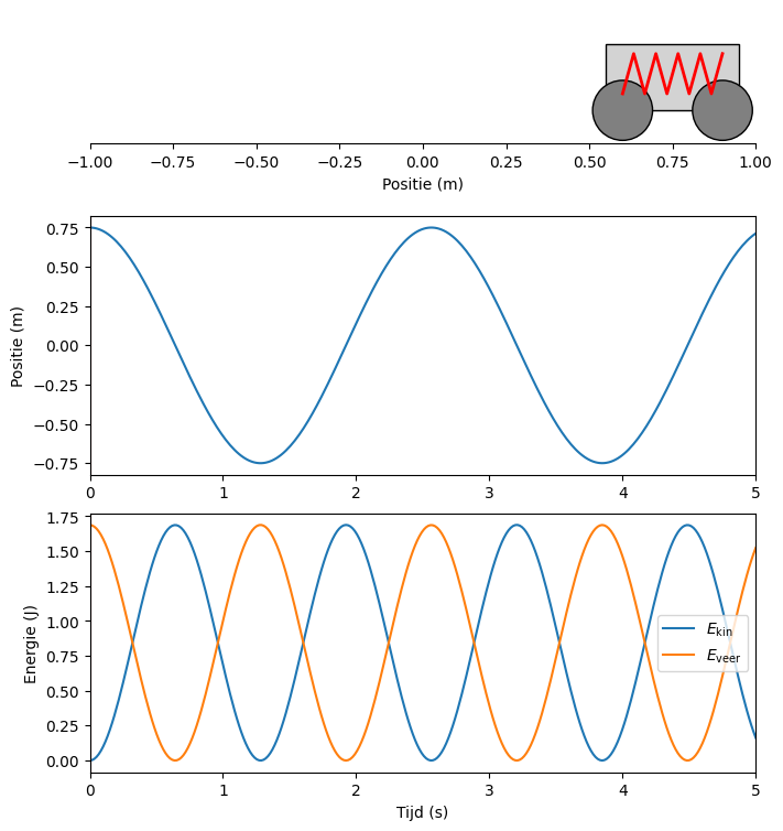
def create_animation(
    t: np.ndarray,
    states: np.ndarray,
    params: dict,
    interval: int = 30,
) -> FuncAnimation:
    """
    Build and return a matplotlib.animation.FuncAnimation.
    If save_path is truthy, attempt to save the animation to that path (mp4).
    """
    # Prepare figure and axes (3 rows)
    fig, ax = plt.subplots(3, 1, figsize=(7, 8), constrained_layout=True)

    # Top: cart and spring
    ax[0].set_yticks([])
    ax[0].set_xlim(-1, 1)
    ax[0].set_ylim(0, 0.4)
    for spine in ("top", "left", "right"):
        ax[0].spines[spine].set_visible(False)
    ax[0].set_xlabel("Positie (m)")

    # Initial positions
    x0 = states[0, 0]

    # Artists
    kar = Rectangle((x0 - 0.2, 0.1), 0.4, 0.2, fc="lightgrey", ec="k")
    wiel1 = Circle((x0 - 0.15, 0.1), 0.09, fc="grey", ec="black")
    wiel2 = Circle((x0 + 0.15, 0.1), 0.09, fc="grey", ec="black")
    spring_x = np.linspace(x0 - 0.15, x0 + abs(x0 * 0.6) - 0.15, 10)
    spring_y = np.tile([0.15, 0.27], len(spring_x) // 2)
    spring_line, = ax[0].plot(spring_x, spring_y, color="red", lw=2)
    ax[0].add_patch(kar)
    ax[0].add_patch(wiel1)
    ax[0].add_patch(wiel2)
    ax[0].set_aspect("equal")

    # Middle: position vs time
    ax[1].plot(t, states[0, :], color="C0")
    ax[1].set_ylabel("Positie (m)")
    pos_vline = ax[1].axvline(t[0], color="red")

    # Bottom: energies
    Ekin_vals, Epot_vals = compute_energies(states, params)
    ax[2].sharex(ax[1])
    ax[2].plot(t, Ekin_vals, label=r"$E_{\mathrm{kin}}$")
    ax[2].plot(t, Epot_vals, label=r"$E_{\mathrm{veer}}$")
    energy_vline = ax[2].axvline(t[0], color="red")
    ax[2].set_xlabel("Tijd (s)")
    ax[2].set_ylabel("Energie (J)")
    ax[2].set_xlim(t[0], t[-1])
    ax[2].legend()

    def update(frame: int):
        x = states[0, frame]
        # use small factor to visualise spring extension
        u = abs(x * 0.4)

        # move body
        kar.set_xy((x - 0.2, 0.1))
        # move wheels
        wiel1.center = (x - 0.15, 0.1)
        wiel2.center = (x + 0.15, 0.1)
        # update spring line
        new_x = np.linspace(x - 0.15, x + u - 0.15, 10)
        new_y = np.tile([0.15, 0.27], len(new_x) // 2)
        spring_line.set_data(new_x, new_y)

        # move vertical time markers
        tnow = t[frame]
        pos_vline.set_xdata([tnow, tnow])
        energy_vline.set_xdata([tnow, tnow])

        return [kar, wiel1, wiel2, spring_line, pos_vline, energy_vline]

    anim = FuncAnimation(fig, update, frames=len(t), interval=interval, blit=True)

    return anim